PIL
- RGB로 이미지를 읽어와서 torchvision 바로 사용 가능.
-
torchvision이 어디서 쓰이길래? -> Pytorch 프레임워크에서 쓰기 위한 데이터 변환이 바로 됌.
PIL 객체를 통해 Numpy로 변환했을 경우 “H x W x C” 형태
“H x W x C” -> “C x H x W” 형태로 변환
이미지 픽셀 값 범위를 0 ~ 255 -> 0 ~ 1로 변환해주기 위해 아래 메소드 사용import torchvision torchvision.transforms.ToTensor()
-
- numpy array와의 암묵적 casting이 되지 않아서 numpy array를 Image array로 변경해줘야 함
Numpy to Tensor
torch.from_numpy(ndarray:numpy.ndarray)
Tensor to Numpy
tensor_data.numpy()
Tensor to Image(png, jpg)
torchvision.utils.save_image(tensor, fp)
Tensor to PILImage
import torchvision.transforms as T

trans = T.TOPILImage()
image_data = trans(tensor_data)
OpenCV
- OpenCV는 BGR로 읽어옴
- 이미지 처리에 필요한 거의 모든 함수 지원
- numpy array 인덱싱을 이용해 직관적인 이미지 전처리 가능
- Video capture 같은 기능의 지원이 잘 되어 있음
마스킹(Masking)
마스킹 작업을 하기 전 각 픽셀들의 데이터 타입을 uint8로 지정해주는 것이 좋다.
import numpy as np

# Numpy의 경우
arr = arr.astype(np.uint8)
이미지 임계처리
Simple thresholding
특정 기준치 넘기면 지정해둔 maxvalue로 값 치환
import cv2
import numpy as np
from matplotlib import pyplot as plt

img = cv2.imread('gradient.jpg',0)

ret, thresh1 = cv2.threshold(img,127,255, cv2.THRESH_BINARY)
ret, thresh2 = cv2.threshold(img,127,255, cv2.THRESH_BINARY_INV)
ret, thresh3 = cv2.threshold(img,127,255, cv2.THRESH_TRUNC)
ret, thresh4 = cv2.threshold(img,127,255, cv2.THRESH_TOZERO)
ret, thresh5 = cv2.threshold(img,127,255, cv2.THRESH_TOZERO_INV)

titles =['Original','BINARY','BINARY_INV','TRUNC','TOZERO','TOZERO_INV']
images = [img,thresh1,thresh2,thresh3,thresh4,thresh5]

for i in xrange(6):
    plt.subplot(2,3,i+1),plt.imshow(images[i],'gray')
    plt.title(titles[i])
    plt.xticks([]),plt.yticks([])

plt.show()
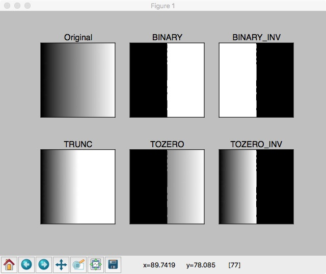
위 그림에서 볼 수 있듯 thresholding type 파라미터를 활용하여 이진화가 아닌 gradual한 이미지 출력도 가능하다.
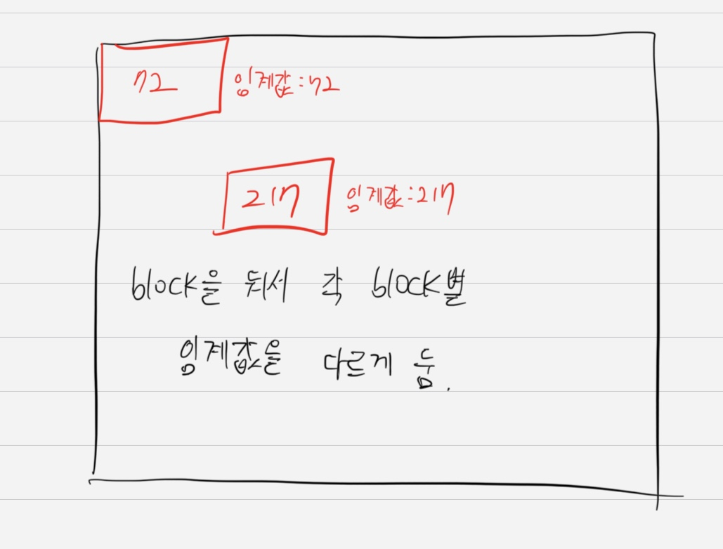
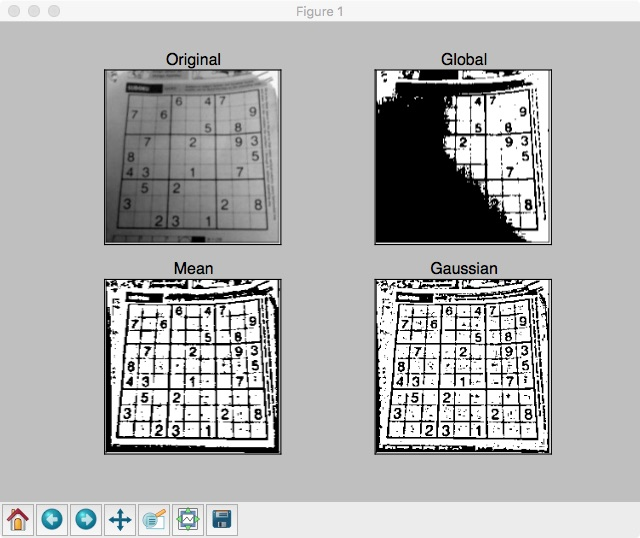
Adaptive thresholding
이미지별로 빛의 세기, 분포가 다르기에 threshold 입력된 이미지마다 적절히 주기 위함
import cv2
import numpy as np
from matplotlib import pyplot as plt

img = cv2.imread('images/dave.png',0)
# img = cv2.medianBlur(img,5)

ret, th1 = cv2.threshold(img,127,255,cv2.THRESH_BINARY)


th2 = cv2.adaptiveThreshold(img,255,cv2.ADAPTIVE_THRESH_MEAN_C,\
cv2.THRESH_BINARY,15,2)
th3 = cv2.adaptiveThreshold(img,255,cv2.ADAPTIVE_THRESH_GAUSSIAN_C,\
cv2.THRESH_BINARY,15,2)

titles = ['Original','Global','Mean','Gaussian']

images = [img,th1,th2,th3]

for i in xrange(4):
    plt.subplot(2,2,i+1),plt.imshow(images[i],'gray')
    plt.title(titles[i])
    plt.xticks([]),plt.yticks([])

plt.show()
Otsu binarization
히스토그램에서 2개의 peak가 있는 이미지가 있을 경우 이진화를 위한 threshold 값을 상당히 정확하게 구해줌
import cv2
import numpy as np
from matplotlib import pyplot as plt

img = cv2.imread('images/noise.png',0)

# global thresholding
ret1, th1 = cv2.threshold(img, 127, 255, cv2.THRESH_BINARY)

ret2, th2 = cv2.threshold(img, 0, 255, cv2.THRESH_BINARY+cv2.THRESH_OTSU)

blur = cv2.GaussianBlur(img,(5,5),0)

ret3, th3 = cv2.threshold(img, 0, 255, cv2.THRESH_BINARY+cv2.THRESH_OTSU)

# plot all the images and their histograms
images = [img, 0, th1, img, 0, th2, blur, 0, th3]

titles = ['Original Noisy Image','Histogram','Global Thresholding (v=127)', 'Original Noisy Image','Histogram',"Otsu's Thresholding", 'Gaussian filtered Image','Histogram',"Otsu's Thresholding"]

for i in xrange(3):
    plt.subplot(3,3,i*3+1),plt.imshow(images[i*3],'gray')
    plt.title(titles[i*3]), plt.xticks([]), plt.yticks([])
    plt.subplot(3,3,i*3+2),plt.hist(images[i*3].ravel(),256)
    plt.title(titles[i*3+1]), plt.xticks([]), plt.yticks([])
    plt.subplot(3,3,i*3+3),plt.imshow(images[i*3+2],'gray')
    plt.title(titles[i*3+2]), plt.xticks([]), plt.yticks([])

plt.show()
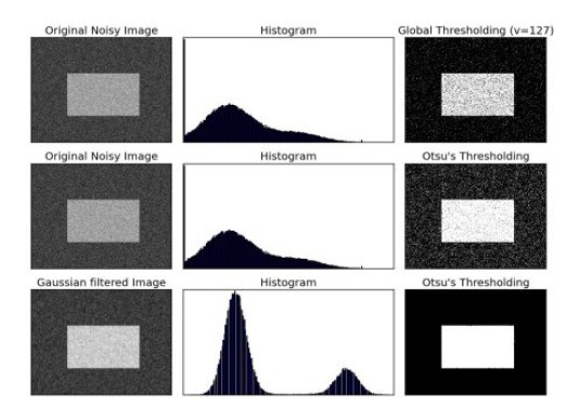
위 그림의 마지막 row는 noise를 gausian blur를 활용해 제거한 뒤 otsu 이진화를 진행한것이다.
바운딩박스 좌표 읽어서 이미지 자르는 예시
import json

def get_coor_from_json(path):
    with open(path) as f:
        raw_data = json.load(f)
        print(raw_data)

    return raw_data['shapes'][0]['points']


box_coor = get_coor_from_json('./cat1.json')    #[[x1, y1], [x2, y2]]

img = Image.open('./data/cat1.jpg')

x1,y1,x2,y2 = box_coor[0][0], box_coor[0][1], box_coor[1][0], box_coor[1][1]
print(x1, y1, x2, y2)
img = img.crop([x1, y1, x2, y2])
img.show()
{'version': '5.0.1', 'flags': {}, 'shapes': [{'label': 'normal', 'points': [[171.99999999999997, 46.666666666666664], [333.8181818181818, 172.72727272727272]], 'group_id': None, 'shape_type': 'rectangle', 'flags': {}}], 'imagePath': 'data\\cat1.jpg', 'imageData': None, 'imageHeight': 408, 'imageWidth': 612}
171.99999999999997 46.666666666666664 333.8181818181818 172.72727272727272
img = Image.open('./data/cat1.jpg')

width, height = img.size

img = img.crop([0,0,width/2,height/2])
img.show()
PREVIOUS경제