사이킷런 LinearRegression을 이용한 보스턴 주택 가격 예측
문제
- 주택 가격을 Regression으로 예측하는 것
- 데이터는 scikit-learn 패키지에 있는 boston 데이터 사용
import numpy as np
import matplotlib.pyplot as plt
import pandas as pd
import seaborn as sns
from scipy import stats
from sklearn.datasets import load_boston
%matplotlib inline

# boston 데이타셋 로드
boston = load_boston()

# boston 데이타셋 DataFrame 변환
bostonDF = pd.DataFrame(boston.data , columns = boston.feature_names)       # boston.data는 feature data들만 반환함
                                                                            # 레이블은 boston.target으로 얻을 수 있음

# boston dataset의 target array는 주택 가격임. 이를 PRICE 컬럼으로 DataFrame에 추가함.
bostonDF['PRICE'] = boston.target

print('Boston 데이타셋 크기 :',bostonDF.shape)
bostonDF.head()
Boston 데이타셋 크기 : (506, 14)


C:\Users\hojun_window\anaconda3\envs\ml\lib\site-packages\sklearn\utils\deprecation.py:87: FutureWarning: Function load_boston is deprecated; `load_boston` is deprecated in 1.0 and will be removed in 1.2.

    The Boston housing prices dataset has an ethical problem. You can refer to
    the documentation of this function for further details.

    The scikit-learn maintainers therefore strongly discourage the use of this
    dataset unless the purpose of the code is to study and educate about
    ethical issues in data science and machine learning.

    In this special case, you can fetch the dataset from the original
    source::

        import pandas as pd
        import numpy as np


        data_url = "http://lib.stat.cmu.edu/datasets/boston"
        raw_df = pd.read_csv(data_url, sep="\s+", skiprows=22, header=None)
        data = np.hstack([raw_df.values[::2, :], raw_df.values[1::2, :2]])
        target = raw_df.values[1::2, 2]

    Alternative datasets include the California housing dataset (i.e.
    :func:`~sklearn.datasets.fetch_california_housing`) and the Ames housing
    dataset. You can load the datasets as follows::

        from sklearn.datasets import fetch_california_housing
        housing = fetch_california_housing()

    for the California housing dataset and::

        from sklearn.datasets import fetch_openml
        housing = fetch_openml(name="house_prices", as_frame=True)

    for the Ames housing dataset.

  warnings.warn(msg, category=FutureWarning)
| CRIM | ZN | INDUS | CHAS | NOX | RM | AGE | DIS | RAD | TAX | PTRATIO | B | LSTAT | PRICE | |
|---|---|---|---|---|---|---|---|---|---|---|---|---|---|---|
| 0 | 0.00632 | 18.0 | 2.31 | 0.0 | 0.538 | 6.575 | 65.2 | 4.0900 | 1.0 | 296.0 | 15.3 | 396.90 | 4.98 | 24.0 |
| 1 | 0.02731 | 0.0 | 7.07 | 0.0 | 0.469 | 6.421 | 78.9 | 4.9671 | 2.0 | 242.0 | 17.8 | 396.90 | 9.14 | 21.6 |
| 2 | 0.02729 | 0.0 | 7.07 | 0.0 | 0.469 | 7.185 | 61.1 | 4.9671 | 2.0 | 242.0 | 17.8 | 392.83 | 4.03 | 34.7 |
| 3 | 0.03237 | 0.0 | 2.18 | 0.0 | 0.458 | 6.998 | 45.8 | 6.0622 | 3.0 | 222.0 | 18.7 | 394.63 | 2.94 | 33.4 |
| 4 | 0.06905 | 0.0 | 2.18 | 0.0 | 0.458 | 7.147 | 54.2 | 6.0622 | 3.0 | 222.0 | 18.7 | 396.90 | 5.33 | 36.2 |
- CRIM: 지역별 범죄 발생률
- ZN: 25,000평방피트를 초과하는 거주 지역의 비율
- NDUS: 비상업 지역 넓이 비율
- CHAS: 찰스강에 대한 더미 변수(강의 경계에 위치한 경우는 1, 아니면 0)
- NOX: 일산화질소 농도
- RM: 거주할 수 있는 방 개수
- AGE: 1940년 이전에 건축된 소유 주택의 비율
- DIS: 5개 주요 고용센터까지의 가중 거리
- RAD: 고속도로 접근 용이도
- TAX: 10,000달러당 재산세율
- PTRATIO: 지역의 교사와 학생 수 비율
- B: 지역의 흑인 거주 비율
- LSTAT: 하위 계층의 비율
-
MEDV: 본인 소유의 주택 가격(중앙값)
- 각 컬럼별로 주택가격에 미치는 영향도를 조사
bostonDF.info()
<class 'pandas.core.frame.DataFrame'>
RangeIndex: 506 entries, 0 to 505
Data columns (total 14 columns):
 #   Column   Non-Null Count  Dtype
---  ------   --------------  -----
 0   CRIM     506 non-null    float64
 1   ZN       506 non-null    float64
 2   INDUS    506 non-null    float64
 3   CHAS     506 non-null    float64
 4   NOX      506 non-null    float64
 5   RM       506 non-null    float64
 6   AGE      506 non-null    float64
 7   DIS      506 non-null    float64
 8   RAD      506 non-null    float64
 9   TAX      506 non-null    float64
 10  PTRATIO  506 non-null    float64
 11  B        506 non-null    float64
 12  LSTAT    506 non-null    float64
 13  PRICE    506 non-null    float64
dtypes: float64(14)
memory usage: 55.5 KB
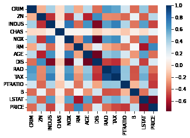
회귀 문제에서의 상관관계 그래프 출력
Heatmap을 통한 correlation matrix 출력
pic = bostonDF.corr()
sns.heatmap(pic, cmap='RdBu')
<AxesSubplot:>
regplot을 이용한 상관관계 출력
# 2개의 행과 4개의 열을 가진 subplots를 이용. axs는 4x2개의 ax를 가짐.
fig, axs = plt.subplots(figsize=(16,8) , ncols=4 , nrows=2)
lm_features = ['RM','ZN','INDUS','NOX','AGE','PTRATIO','LSTAT','RAD']
for i , feature in enumerate(lm_features):
    row = int(i/4)
    col = i%4
    # 시본의 regplot을 이용해 산점도와 선형 회귀 직선을 함께 표현
    sns.regplot(x=feature , y='PRICE',data=bostonDF , ax=axs[row][col])
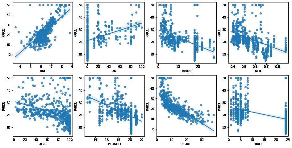
- regplot보다 heatmap을 통해서 상관관계를 보는것이 더 편한듯 하다
학습과 테스트 데이터 세트로 분리하고 학습/예측/평가 수행
from sklearn.model_selection import train_test_split
from sklearn.linear_model import LinearRegression
from sklearn.metrics import mean_squared_error , r2_score

y_target = bostonDF['PRICE']
X_data = bostonDF.drop(['PRICE'],axis=1,inplace=False)

X_train , X_test , y_train , y_test = train_test_split(X_data , y_target ,test_size=0.3, random_state=156)

# Linear Regression OLS로 학습/예측/평가 수행.
lr = LinearRegression()
lr.fit(X_train ,y_train )
y_preds = lr.predict(X_test)
mse = mean_squared_error(y_test, y_preds)
rmse = np.sqrt(mse)

print('MSE : {0:.3f} , RMSE : {1:.3F}'.format(mse , rmse))
print('Variance score : {0:.3f}'.format(r2_score(y_test, y_preds)))
MSE : 17.297 , RMSE : 4.159
Variance score : 0.757
print('절편 값:',lr.intercept_)
print('회귀 계수값:', np.round(lr.coef_, 1))
절편 값: 40.995595172164336
회귀 계수값: [ -0.1   0.1   0.    3.  -19.8   3.4   0.   -1.7   0.4  -0.   -0.9   0.
  -0.6]
# 회귀 계수를 큰 값 순으로 정렬하기 위해 Series로 생성. index가 컬럼명에 유의
coeff = pd.Series(data=np.round(lr.coef_, 1), index=X_data.columns )
coeff.sort_values(ascending=False)
RM          3.4
CHAS        3.0
RAD         0.4
ZN          0.1
INDUS       0.0
AGE         0.0
TAX        -0.0
B           0.0
CRIM       -0.1
LSTAT      -0.6
PTRATIO    -0.9
DIS        -1.7
NOX       -19.8
dtype: float64
- RM이 양의 값으로 가장 큰 회귀 계수를 가지며, NOX는 음의 값으로 가장 큰 회귀 계수를 갖는다
from sklearn.model_selection import cross_val_score

y_target = bostonDF['PRICE']
X_data = bostonDF.drop(['PRICE'],axis=1,inplace=False)
lr = LinearRegression()

# cross_val_score( )로 5 Fold 셋으로 MSE 를 구한 뒤 이를 기반으로 다시  RMSE 구함.
neg_mse_scores = cross_val_score(lr, X_data, y_target, scoring="neg_mean_squared_error", cv = 5)
rmse_scores  = np.sqrt(-1 * neg_mse_scores)
avg_rmse = np.mean(rmse_scores)

# cross_val_score(scoring="neg_mean_squared_error")로 반환된 값은 모두 음수
print(' 5 folds 의 개별 Negative MSE scores: ', np.round(neg_mse_scores, 2))
print(' 5 folds 의 개별 RMSE scores : ', np.round(rmse_scores, 2))
print(' 5 folds 의 평균 RMSE : {0:.3f} '.format(avg_rmse))
 5 folds 의 개별 Negative MSE scores:  [-12.46 -26.05 -33.07 -80.76 -33.31]
 5 folds 의 개별 RMSE scores :  [3.53 5.1  5.75 8.99 5.77]
 5 folds 의 평균 RMSE : 5.829
과적합 되어있지 않는지 확인해보기 위해 규제(Regularization)를 적용해보자
릿지 회귀(L2 Norm 활용)
# 앞의 LinearRegression예제에서 분할한 feature 데이터 셋인 X_data과 Target 데이터 셋인 Y_target 데이터셋을 그대로 이용
from sklearn.linear_model import Ridge
from sklearn.model_selection import cross_val_score

# boston 데이타셋 로드
boston = load_boston()

# boston 데이타셋 DataFrame 변환
bostonDF = pd.DataFrame(boston.data , columns = boston.feature_names)

# boston dataset의 target array는 주택 가격임. 이를 PRICE 컬럼으로 DataFrame에 추가함.
bostonDF['PRICE'] = boston.target
print('Boston 데이타셋 크기 :',bostonDF.shape)

y_target = bostonDF['PRICE']
X_data = bostonDF.drop(['PRICE'],axis=1,inplace=False)

ridge = Ridge(alpha = 10)
neg_mse_scores = cross_val_score(ridge, X_data, y_target, scoring="neg_mean_squared_error", cv = 5)
rmse_scores  = np.sqrt(-1 * neg_mse_scores)
avg_rmse = np.mean(rmse_scores)
print(' 5 folds 의 개별 Negative MSE scores: ', np.round(neg_mse_scores, 3))
print(' 5 folds 의 개별 RMSE scores : ', np.round(rmse_scores,3))
print(' 5 folds 의 평균 RMSE : {0:.3f} '.format(avg_rmse))
Boston 데이타셋 크기 : (506, 14)
 5 folds 의 개별 Negative MSE scores:  [-11.422 -24.294 -28.144 -74.599 -28.517]
 5 folds 의 개별 RMSE scores :  [3.38  4.929 5.305 8.637 5.34 ]
 5 folds 의 평균 RMSE : 5.518
- 규제 적용 전 보다 약간 개선된 효과를 얻음
각 alpha에 따른 회귀 계수 값을 시각화. 각 alpha값 별로 plt.subplots로 맷플롯립 축 생성
# 각 alpha에 따른 회귀 계수 값을 시각화하기 위해 5개의 열로 된 맷플롯립 축 생성
fig , axs = plt.subplots(figsize=(18,6) , nrows=1 , ncols=5)
# 각 alpha에 따른 회귀 계수 값을 데이터로 저장하기 위한 DataFrame 생성
coeff_df = pd.DataFrame()

# alphas 리스트 값을 차례로 입력해 회귀 계수 값 시각화 및 데이터 저장. pos는 axis의 위치 지정
for pos , alpha in enumerate(alphas) :
    ridge = Ridge(alpha = alpha)
    ridge.fit(X_data , y_target)
    # alpha에 따른 피처별 회귀 계수를 Series로 변환하고 이를 DataFrame의 컬럼으로 추가.
    coeff = pd.Series(data=ridge.coef_ , index=X_data.columns )
    colname='alpha:'+str(alpha)
    coeff_df[colname] = coeff
    # 막대 그래프로 각 alpha 값에서의 회귀 계수를 시각화. 회귀 계수값이 높은 순으로 표현
    coeff = coeff.sort_values(ascending=False)
    axs[pos].set_title(colname)
    axs[pos].set_xlim(-3,6)
    sns.barplot(x=coeff.values , y=coeff.index, ax=axs[pos])

# for 문 바깥에서 맷플롯립의 show 호출 및 alpha에 따른 피처별 회귀 계수를 DataFrame으로 표시
plt.show()
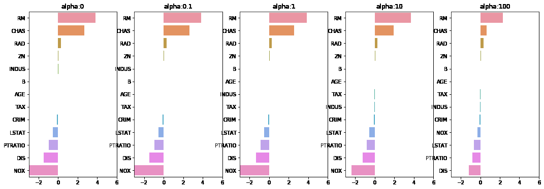
- alpha 값이 증가할수록 피쳐 계수들의 값(W)이 줄어듬을 확인
- subplot과 seaborn이 ax 인자로 연계될 수 있는것도 주목하면 좋을 듯
alpha 값에 따른 컬럼별 회귀계수 출력
ridge_alphas = [0 , 0.1 , 1 , 10 , 100]
sort_column = 'alpha:'+str(ridge_alphas[0])
coeff_df.sort_values(by=sort_column, ascending=False)
| alpha:0 | alpha:0.1 | alpha:1 | alpha:10 | alpha:100 | |
|---|---|---|---|---|---|
| RM | 3.809865 | 3.818233 | 3.854000 | 3.702272 | 2.334536 |
| CHAS | 2.686734 | 2.670019 | 2.552393 | 1.952021 | 0.638335 |
| RAD | 0.306049 | 0.303515 | 0.290142 | 0.279596 | 0.315358 |
| ZN | 0.046420 | 0.046572 | 0.047443 | 0.049579 | 0.054496 |
| INDUS | 0.020559 | 0.015999 | -0.008805 | -0.042962 | -0.052826 |
| B | 0.009312 | 0.009368 | 0.009673 | 0.010037 | 0.009393 |
| AGE | 0.000692 | -0.000269 | -0.005415 | -0.010707 | 0.001212 |
| TAX | -0.012335 | -0.012421 | -0.012912 | -0.013993 | -0.015856 |
| CRIM | -0.108011 | -0.107474 | -0.104595 | -0.101435 | -0.102202 |
| LSTAT | -0.524758 | -0.525966 | -0.533343 | -0.559366 | -0.660764 |
| PTRATIO | -0.952747 | -0.940759 | -0.876074 | -0.797945 | -0.829218 |
| DIS | -1.475567 | -1.459626 | -1.372654 | -1.248808 | -1.153390 |
| NOX | -17.766611 | -16.684645 | -10.777015 | -2.371619 | -0.262847 |
라쏘 회귀(L1 Norm 활용)
from sklearn.linear_model import Lasso, ElasticNet

# alpha값에 따른 회귀 모델의 폴드 평균 RMSE를 출력하고 회귀 계수값들을 DataFrame으로 반환
def get_linear_reg_eval(model_name, params=None, X_data_n=None, y_target_n=None,
                        verbose=True, return_coeff=True):
    coeff_df = pd.DataFrame()
    if verbose : print('####### ', model_name , '#######')
    for param in params:
        if model_name =='Ridge': model = Ridge(alpha=param)
        elif model_name =='Lasso': model = Lasso(alpha=param)
        elif model_name =='ElasticNet': model = ElasticNet(alpha=param, l1_ratio=0.7)
        neg_mse_scores = cross_val_score(model, X_data_n,
                                             y_target_n, scoring="neg_mean_squared_error", cv = 5)
        avg_rmse = np.mean(np.sqrt(-1 * neg_mse_scores))
        print('alpha {0}일 때 5 폴드 세트의 평균 RMSE: {1:.3f} '.format(param, avg_rmse))
        # cross_val_score는 evaluation metric만 반환하므로 모델을 다시 학습하여 회귀 계수 추출

        model.fit(X_data_n , y_target_n)
        if return_coeff:
            # alpha에 따른 피처별 회귀 계수를 Series로 변환하고 이를 DataFrame의 컬럼으로 추가.
            coeff = pd.Series(data=model.coef_ , index=X_data_n.columns )
            colname='alpha:'+str(param)
            coeff_df[colname] = coeff

    return coeff_df
# end of get_linear_regre_eval
# 라쏘에 사용될 alpha 파라미터의 값들을 정의하고 get_linear_reg_eval() 함수 호출
lasso_alphas = [ 0.07, 0.1, 0.5, 1, 3]
coeff_lasso_df =get_linear_reg_eval('Lasso', params=lasso_alphas, X_data_n=X_data, y_target_n=y_target)
#######  Lasso #######
alpha 0.07일 때 5 폴드 세트의 평균 RMSE: 5.612
alpha 0.1일 때 5 폴드 세트의 평균 RMSE: 5.615
alpha 0.5일 때 5 폴드 세트의 평균 RMSE: 5.669
alpha 1일 때 5 폴드 세트의 평균 RMSE: 5.776
alpha 3일 때 5 폴드 세트의 평균 RMSE: 6.189
# 반환된 coeff_lasso_df를 첫번째 컬럼순으로 내림차순 정렬하여 회귀계수 DataFrame출력
sort_column = 'alpha:'+str(lasso_alphas[0])
coeff_lasso_df.sort_values(by=sort_column, ascending=False)
| alpha:0.07 | alpha:0.1 | alpha:0.5 | alpha:1 | alpha:3 | |
|---|---|---|---|---|---|
| RM | 3.789725 | 3.703202 | 2.498212 | 0.949811 | 0.000000 |
| CHAS | 1.434343 | 0.955190 | 0.000000 | 0.000000 | 0.000000 |
| RAD | 0.270936 | 0.274707 | 0.277451 | 0.264206 | 0.061864 |
| ZN | 0.049059 | 0.049211 | 0.049544 | 0.049165 | 0.037231 |
| B | 0.010248 | 0.010249 | 0.009469 | 0.008247 | 0.006510 |
| NOX | -0.000000 | -0.000000 | -0.000000 | -0.000000 | 0.000000 |
| AGE | -0.011706 | -0.010037 | 0.003604 | 0.020910 | 0.042495 |
| TAX | -0.014290 | -0.014570 | -0.015442 | -0.015212 | -0.008602 |
| INDUS | -0.042120 | -0.036619 | -0.005253 | -0.000000 | -0.000000 |
| CRIM | -0.098193 | -0.097894 | -0.083289 | -0.063437 | -0.000000 |
| LSTAT | -0.560431 | -0.568769 | -0.656290 | -0.761115 | -0.807679 |
| PTRATIO | -0.765107 | -0.770654 | -0.758752 | -0.722966 | -0.265072 |
| DIS | -1.176583 | -1.160538 | -0.936605 | -0.668790 | -0.000000 |
- 주목할만한 점
- 릿지 회귀(L2 norm)은 W 회귀계수 크기를 줄일 뿐 W 요소들을 0으로 만들지는 않음
- 라쏘 회귀(L1 norm)은 W 요소들을 0으로 만들기도 함. (불필요한 피쳐 제거)
엘라스틱넷 회귀
PREVIOUS경제