NLP와 텍스트 분석의 차이
- NLP
- 텍스트 분석을 향상하게 하는 기반 기술
- 기계 번역, 자동으로 질문을 해석하고 답해주는 자동 응답 시스템 등
- 텍스트 분석
- 텍스트 마이닝이라고도 불림
- 비정형 텍스트에서 의미있는 정보를 추출하는 것
- 크게 4개의 기술영역 존재
- 텍스트 분류
- 감성 분석
- 텍스트 요약
- 텍스트 군집화와 유사도 측정
데이터 전처리
- 숫자형 데이터는 그 자체로 의미있는 값이 되는 경우가 대부분이지만 텍스트 데이터는 그렇지 않음. 즉 의미있는 피처 형태로 추출해야함. 다시 말하자면 전처리가 좀 빡셈
- 클렌징, 대/소문자 변경, 특수문자 삭제, 단어 토큰화, 의미없는 단어 제거, 어근 추출 등의 전처리 필요
클렌징
- 텍스트 분석에서 방해가 되는 불필요한 문자, 기호등을 사전에 제거하는 작업. html, xml 태그 같은것 지우는 작업
텍스트 토큰화
- 파이썬
NLTK라이브러리에서 지원- 문서에서 문장을 토큰으로 분리하는 문장 토큰화. 문장의 마침표(.), 개행문자(\n)등 문장의 마지막을 뜻하는 기호에 따라 분리하는것이 일반적
from nltk import sent_tokenize
import nltk
nltk.download('punkt')

text_sample = 'The Matrix is everywhere its all around us, here even in this room. \
            You can see it out your window or on your television. \
            You feel it when you go to work, or go to church or pay your taxes.'

sentences = sent_tokenize(text=text_sample)
print(type(sentences),len(sentences))
print(sentences)
<class 'list'> 3 ['The Matrix is everywhere its all around us, here even in this room.', 'You can see it out your window or on your television.', 'You feel it when you go to work, or go to church or pay your taxes.'] [nltk_data] Downloading package punkt to [nltk_data] C:\Users\hojun_window\AppData\Roaming\nltk_data... [nltk_data] Package punkt is already up-to-date! - 문장에서 단어를 토큰으로 분리하는 단어 토큰화. 공백, 콤바(,), 마침표(.), 개행문자 등으로 단어 분리 가능하며 정규 표현식으로도 가능
-
문장 토큰화, 단어 토큰화 동시에 사용해보자
from nltk import word_tokenize, sent_tokenize

#여러개의 문장으로 된 입력 데이터를 문장별로 단어 토큰화 만드는 함수 생성
def tokenize_text(text):

    # 문장별로 분리 토큰
    sentences = sent_tokenize(text)

    # workd_tokens = []
    # for sentence in sentences:
    #     word_tokens.append(word_tokenize(temp))

    # 분리된 문장별 단어 토큰화
    word_tokens = [word_tokenize(sentence) for sentence in sentences]   # 위 주석한 for문과 이 코드는 완전히 같은 코드
                                                                        # 리스트 컴프리헨션!
    return word_tokens

#여러 문장들에 대해 문장별 단어 토큰화 수행.
word_tokens = tokenize_text(text_sample)
print(type(word_tokens),len(word_tokens))
print(word_tokens)
<class 'list'> 3 [['The', 'Matrix', 'is', 'everywhere', 'its', 'all', 'around', 'us', ',', 'here', 'even', 'in', 'this', 'room', '.'], ['You', 'can', 'see', 'it', 'out', 'your', 'window', 'or', 'on', 'your', 'television', '.'], ['You', 'feel', 'it', 'when', 'you', 'go', 'to', 'work', ',', 'or', 'go', 'to', 'church', 'or', 'pay', 'your', 'taxes', '.']]- 위와같이 구성요소를 모두 단어단위로 토큰화하면 문맥적 의미가 사라짐(단어가 붙어서 새로운 의미를 만드는 경우를 고려 불가함)
- 해결방안은 N-gram! -> 연속된 n 개의 단어를 하나의 토큰화 단위로 분리해 내는것
- “Agent Smith knock the door” 문장이 있을 시 이를 2-gram으로 만들면 (Agent, Smith), (Smith, knock), (knock, the), (the, door)로 토큰화 됨
- N-gram을 활용한 자연어 처리 모델 평가 실습코드는 BLEU 기반 문장 평가에서 확인 가능
- 문서에서 문장을 토큰으로 분리하는 문장 토큰화. 문장의 마침표(.), 개행문자(\n)등 문장의 마지막을 뜻하는 기호에 따라 분리하는것이 일반적
스톱 워드 제거
- is, the, a, will 같이 영어에서 굉장히 자주 나오는 단어는 사실 중요하지 않지만 그 빈도수로 인해 중요하게 인식 될 가능성이 높으며 이러한 단어를 제거해주는 작업
import nltk

stopwords = nltk.corpus.stopwords.words('english')
all_tokens = []

# 위 예제의 3개의 문장별로 얻은 word_tokens list 에 대해 stop word 제거 Loop
# for sentence in word_tokens:
#     filtered_words=[]
#     # 개별 문장별로 tokenize된 sentence list에 대해 stop word 제거 Loop
#     for word in sentence:
#         #소문자로 모두 변환합니다.
#         word = word.lower()
#         # tokenize 된 개별 word가 stop words 들의 단어에 포함되지 않으면 word_tokens에 추가
#         if word not in stopwords:
#             filtered_words.append(word)
#     all_tokens.append(filtered_words)

all_tokens = [word for sentence in word_tokens for word in sentence if word not in stopwords]   # 리스트 컴프리헨션으로 위 코드 재현해봄 ㅎㅎ

print(all_tokens)
['The', 'Matrix', 'everywhere', 'around', 'us', ',', 'even', 'room', '.', 'You', 'see', 'window', 'television', '.', 'You', 'feel', 'go', 'work', ',', 'go', 'church', 'pay', 'taxes', '.']
Stemming, Lemmatization
많은 언어에서 문법적인 요소에 따라 단어가 다양하게 변하며 이는 머신러닝 적용에 방해 요소로 작동할 수 있음 Stemming, Lemmatization은 단어의 원형을 찾아주는 방법임
- Stemming보다 Lemmatization이 더 정확하지만 속도가 느림
- Lemmatization은 단어의 품사까지 입력시켜 줘야함
from nltk.stem import LancasterStemmer
stemmer = LancasterStemmer()

print(stemmer.stem('working'),stemmer.stem('works'),stemmer.stem('worked'))
print(stemmer.stem('amusing'),stemmer.stem('amuses'),stemmer.stem('amused'))
print(stemmer.stem('happier'),stemmer.stem('happiest'))
print(stemmer.stem('fancier'),stemmer.stem('fanciest'))
work work work
amus amus amus
happy happiest
fant fanciest
- amuse가 단어의 원형인데 잘 못 나오는 모습
- happy, fant도 역시 단어의 원형을 잘 잡지 못하고 있음
from nltk.stem import WordNetLemmatizer
import nltk
nltk.download('wordnet')

lemma = WordNetLemmatizer()
print(lemma.lemmatize('amusing','v'),lemma.lemmatize('amuses','v'),lemma.lemmatize('amused','v'))
print(lemma.lemmatize('happier','a'),lemma.lemmatize('happiest','a'))
print(lemma.lemmatize('fancier','a'),lemma.lemmatize('fanciest','a'))
amuse amuse amuse
happy happy
fancy fancy
피처 추출
- 피처 추출 방식은 크게 2가지
-
BOW(Bag of Words)
- 봉투(Bag)안에 단어를 넣어서 흔들어서 섞는다는 의미. 즉 모든 단어를 문맥이나 순서를 무시하고 일괄적으로 단어의 빈도 값을 부여해 피처값 추출하는 모델
- 장점
- 쉽고 빠름
- 단점
- 문맥의미 반영 부족
- N-gram을 통해 문맥의미를 어느정도 반영할 순 있으나 어디까지나 보조수단임
- 희소행렬 문제 발생
- 많은 문장은 서로 다른 언어로 이루어져 있어서 희소행렬 형태가 나타날 가능성이 매우 큼 (희소행렬의 반대말은 밀집행렬)
- 문맥의미 반영 부족
- 2가지 방식 존재
- Count 기반 벡터화
- 말 그대로 단어가 나온 수만 파악하는 것
- TF-IDF 기반 벡터화
- 자주 나타는는 단어에 높은 가중치를 주되, 모든 문서에서 전반적으로 자주 나타나는 언어에 대해선 패널티를 줌
-
\[TFIDF_i = TF_i * log{N \over DF_i}\]
- \(TF_i\): 개별 문서에서의 단어 i 빈도
- \(DF_i\): 단어 i를 가지고 있는 문서 개수
- \(N\): 전체 문서 개수
- Count 기반 벡터화
- 이렇게 Bag를 진행하면 희소행렬이 나오지만 희소행렬 형태일 경우 메모리 낭비가 심함. 이를 위한 처리 방식 2가지 존재
-
COO 형식
- 0이 아닌 데이터들을 배열에 넣고, 그 데이터들의 인덱스도 역시 배열에 넣는 방식
 import numpy as np
 from scipy import sparse
 dense = np.array( [ [ 3, 0, 1 ], [0, 2, 0 ] ] )

 # 0 이 아닌 데이터 추출
 data = np.array([3,1,2])

 # 행 위치와 열 위치를 각각 array로 생성
 row_pos = np.array([0,0,1])
 col_pos = np.array([0,2,1])     # (0,0), (0,2), (1,1)이 각각 3, 1, 2 데이터의 위치

 # sparse 패키지의 coo_matrix를 이용하여 COO 형식으로 희소 행렬 생성
 sparse_coo = sparse.coo_matrix((data, (row_pos,col_pos)))
 sparse_coo, sparse_coo.toarray()
(<2x3 sparse matrix of type '<class 'numpy.int32'>' with 3 stored elements in COOrdinate format>, array([[3, 0, 1], [0, 2, 0]])) -
CSR 형식
 import numpy as np
 dense2 = np.array([
     [0,0,1,0,0,5],
     [1,4,0,3,2,5],
     [0,6,0,3,0,0],
     [2,0,0,0,0,0],
     [0,0,0,7,0,8],
     [1,0,0,0,0,0]])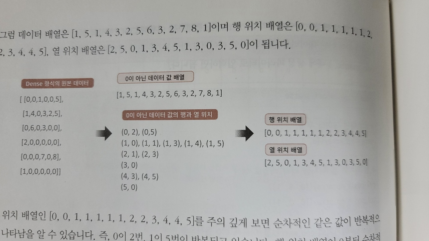
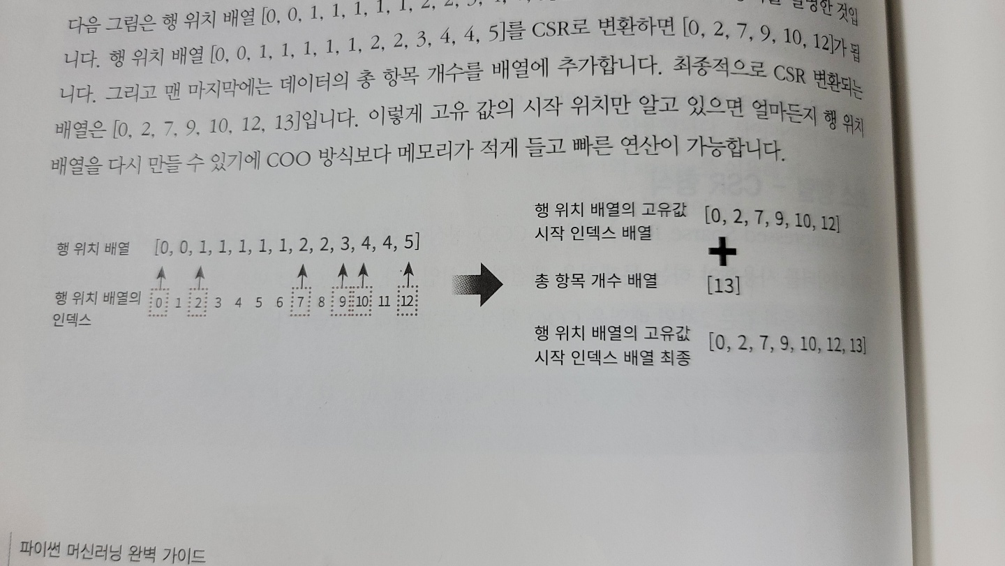
 from scipy import sparse

 dense2 = np.array([[0,0,1,0,0,5],
             [1,4,0,3,2,5],
             [0,6,0,3,0,0],
             [2,0,0,0,0,0],
             [0,0,0,7,0,8],
             [1,0,0,0,0,0]])

 # 0 이 아닌 데이터 추출
 data2 = np.array([1, 5, 1, 4, 3, 2, 5, 6, 3, 2, 7, 8, 1])

 # 행 위치와 열 위치를 각각 array로 생성
 row_pos = np.array([0, 0, 1, 1, 1, 1, 1, 2, 2, 3, 4, 4, 5])
 col_pos = np.array([2, 5, 0, 1, 3, 4, 5, 1, 3, 0, 3, 5, 0])

 # COO 형식으로 변환
 sparse_coo = sparse.coo_matrix((data2, (row_pos,col_pos)))

 # 행 위치 배열의 고유한 값들의 시작 위치 인덱스를 배열로 생성
 row_pos_ind = np.array([0, 2, 7, 9, 10, 12, 13])

 # CSR 형식으로 변환
 sparse_csr = sparse.csr_matrix((data2, col_pos, row_pos_ind))

 print('COO 변환된 데이터가 제대로 되었는지 다시 Dense로 출력 확인')
 print(sparse_coo.toarray())
 print('CSR 변환된 데이터가 제대로 되었는지 다시 Dense로 출력 확인')
 print(sparse_csr.toarray())
COO 변환된 데이터가 제대로 되었는지 다시 Dense로 출력 확인 [[0 0 1 0 0 5] [1 4 0 3 2 5] [0 6 0 3 0 0] [2 0 0 0 0 0] [0 0 0 7 0 8] [1 0 0 0 0 0]] CSR 변환된 데이터가 제대로 되었는지 다시 Dense로 출력 확인 [[0 0 1 0 0 5] [1 4 0 3 2 5] [0 6 0 3 0 0] [2 0 0 0 0 0] [0 0 0 7 0 8] [1 0 0 0 0 0]]
-
실제로 사용할 땐 그냥 희소행렬을 입력으로 넣으면 됨. ()
  dense3 = np.array([[0,0,1,0,0,5],
              [1,4,0,3,2,5],
              [0,6,0,3,0,0],
              [2,0,0,0,0,0],
              [0,0,0,7,0,8],
              [1,0,0,0,0,0]])

  coo = sparse.coo_matrix(dense3)
  csr = sparse.csr_matrix(dense3)
-
Word2Vec
- 향후에 채워넣을 것
실제 뉴스 데이터를 통한 Classification 진행
텍스트 정규화
from sklearn.datasets import fetch_20newsgroups

news_data = fetch_20newsgroups(subset='all',random_state=156)
print(news_data.keys())
dict_keys(['data', 'filenames', 'target_names', 'target', 'DESCR'])
import pandas as pd

print('target 클래스의 값과 분포도 \n',pd.Series(news_data.target).value_counts().sort_index())
print('target 클래스의 이름들 \n',news_data.target_names)
target 클래스의 값과 분포도
 0     799
1     973
2     985
3     982
4     963
5     988
6     975
7     990
8     996
9     994
10    999
11    991
12    984
13    990
14    987
15    997
16    910
17    940
18    775
19    628
dtype: int64
target 클래스의 이름들
 ['alt.atheism', 'comp.graphics', 'comp.os.ms-windows.misc', 'comp.sys.ibm.pc.hardware', 'comp.sys.mac.hardware', 'comp.windows.x', 'misc.forsale', 'rec.autos', 'rec.motorcycles', 'rec.sport.baseball', 'rec.sport.hockey', 'sci.crypt', 'sci.electronics', 'sci.med', 'sci.space', 'soc.religion.christian', 'talk.politics.guns', 'talk.politics.mideast', 'talk.politics.misc', 'talk.religion.misc']
from sklearn.datasets import fetch_20newsgroups

# subset='train'으로 학습용(Train) 데이터만 추출, remove=('headers', 'footers', 'quotes')로 내용만 추출
train_news= fetch_20newsgroups(subset='train', remove=('headers', 'footers', 'quotes'), random_state=156)
X_train = train_news.data
y_train = train_news.target
print(type(X_train))

# subset='test'으로 테스트(Test) 데이터만 추출, remove=('headers', 'footers', 'quotes')로 내용만 추출
test_news= fetch_20newsgroups(subset='test',remove=('headers', 'footers','quotes'),random_state=156)
X_test = test_news.data
y_test = test_news.target
print('학습 데이터 크기 {0} , 테스트 데이터 크기 {1}'.format(len(train_news.data) , len(test_news.data)))
<class 'list'>
학습 데이터 크기 11314 , 테스트 데이터 크기 7532
피처 벡터화 변환과 머신러닝 모델 학습/예측/평가
from sklearn.feature_extraction.text import CountVectorizer

# Count Vectorization으로 feature extraction 변환 수행.
cnt_vect = CountVectorizer()
# 개정판 소스 코드 변경(2019.12.24)
cnt_vect.fit(X_train)
X_train_cnt_vect = cnt_vect.transform(X_train)

# 학습 데이터로 fit( )된 CountVectorizer를 이용하여 테스트 데이터를 feature extraction 변환 수행.
X_test_cnt_vect = cnt_vect.transform(X_test)

print('학습 데이터 Text의 CountVectorizer Shape:',X_train_cnt_vect.shape)
학습 데이터 Text의 CountVectorizer Shape: (11314, 101631)
from sklearn.linear_model import LogisticRegression
from sklearn.metrics import accuracy_score

lrRegression = LogisticRegression()
lrRegression.fit(X_train_cnt_vect, y_train)
pred = lrRegression.predict(X_test_cnt_vect)

accuracy_score(y_test, pred)
C:\Users\hojun_window\anaconda3\envs\ml\lib\site-packages\sklearn\linear_model\_logistic.py:814: ConvergenceWarning: lbfgs failed to converge (status=1):
STOP: TOTAL NO. of ITERATIONS REACHED LIMIT.

Increase the number of iterations (max_iter) or scale the data as shown in:
    https://scikit-learn.org/stable/modules/preprocessing.html
Please also refer to the documentation for alternative solver options:
    https://scikit-learn.org/stable/modules/linear_model.html#logistic-regression
  n_iter_i = _check_optimize_result(


0.6066117896972916
from sklearn.feature_extraction.text import TfidfVectorizer

# TF-IDF Vectorization 적용하여 학습 데이터셋과 테스트 데이터 셋 변환.
tfidf_vect = TfidfVectorizer()
tfidf_vect.fit(X_train)
X_train_tfidf_vect = tfidf_vect.transform(X_train)
print(f'X_train_tfidf_vect shape: {X_train_tfidf_vect.shape}')
X_test_tfidf_vect = tfidf_vect.transform(X_test)

# LogisticRegression을 이용하여 학습/예측/평가 수행.
lr_clf = LogisticRegression()
lr_clf.fit(X_train_tfidf_vect , y_train)
pred = lr_clf.predict(X_test_tfidf_vect)
print('TF-IDF Logistic Regression 의 예측 정확도는 {0:.3f}'.format(accuracy_score(y_test ,pred)))
X_train_tfidf_vect shape: (11314, 101631)
TF-IDF Logistic Regression 의 예측 정확도는 0.674
# stop words 필터링을 추가하고 ngram을 기본(1,1)에서 (1,2)로 변경하여 Feature Vectorization 적용.
tfidf_vect = TfidfVectorizer(stop_words='english', ngram_range=(1,2), max_df=300 )
tfidf_vect.fit(X_train)
X_train_tfidf_vect = tfidf_vect.transform(X_train)
print(f'X_train_tfidf_vect shape: {X_train_tfidf_vect.shape}')
X_test_tfidf_vect = tfidf_vect.transform(X_test)

lr_clf = LogisticRegression()
lr_clf.fit(X_train_tfidf_vect , y_train)
pred = lr_clf.predict(X_test_tfidf_vect)
print('TF-IDF Vectorized Logistic Regression 의 예측 정확도는 {0:.3f}'.format(accuracy_score(y_test ,pred)))
X_train_tfidf_vect shape: (11314, 943453)
TF-IDF Vectorized Logistic Regression 의 예측 정확도는 0.692
from sklearn.model_selection import GridSearchCV

# 최적 C 값 도출 튜닝 수행. CV는 3 Fold셋으로 설정.
params = { 'C':[0.01, 0.1, 1, 5, 10]}
grid_cv_lr = GridSearchCV(lr_clf ,param_grid=params , cv=3 , scoring='accuracy' , verbose=1 )
grid_cv_lr.fit(X_train_tfidf_vect , y_train)
print('Logistic Regression best C parameter :',grid_cv_lr.best_params_ )

# 최적 C 값으로 학습된 grid_cv로 예측 수행하고 정확도 평가.
pred = grid_cv_lr.predict(X_test_tfidf_vect)
print('TF-IDF Vectorized Logistic Regression 의 예측 정확도는 {0:.3f}'.format(accuracy_score(y_test ,pred)))
Fitting 3 folds for each of 5 candidates, totalling 15 fits


[Parallel(n_jobs=1)]: Done  15 out of  15 | elapsed:  4.0min finished


Logistic Regression best C parameter : {'C': 10}
TF-IDF Vectorized Logistic Regression 의 예측 정확도는 0.704
사이킷런 파이프라인(Pipeline) 사용 및 GridSearchCV와의 결합
from sklearn.pipeline import Pipeline

# TfidfVectorizer 객체를 tfidf_vect 객체명으로, LogisticRegression객체를 lr_clf 객체명으로 생성하는 Pipeline생성
pipeline = Pipeline([
    ('tfidf_vect', TfidfVectorizer(stop_words='english', ngram_range=(1,2), max_df=300)),
    ('lr_clf', LogisticRegression(C=10))
])

# 별도의 TfidfVectorizer객체의 fit_transform( )과 LogisticRegression의 fit(), predict( )가 필요 없음.
# pipeline의 fit( ) 과 predict( ) 만으로 한꺼번에 Feature Vectorization과 ML 학습/예측이 가능.
pipeline.fit(X_train, y_train)
pred = pipeline.predict(X_test)
print('Pipeline을 통한 Logistic Regression 의 예측 정확도는 {0:.3f}'.format(accuracy_score(y_test ,pred)))
Pipeline을 통한 Logistic Regression 의 예측 정확도는 0.704
from sklearn.pipeline import Pipeline

pipeline = Pipeline([
    ('tfidf_vect', TfidfVectorizer(stop_words='english')),
    ('lr_clf', LogisticRegression())
])

# Pipeline에 기술된 각각의 객체 변수에 언더바(_)2개를 연달아 붙여 GridSearchCV에 사용될
# 파라미터/하이퍼 파라미터 이름과 값을 설정. .
# 오호라.. 이렇게 pipeline과 GridSearchCV이 연동이 되는구먼! 언더바 2개!
params = { 'tfidf_vect__ngram_range': [(1,1), (1,2), (1,3)],
           'tfidf_vect__max_df': [100, 300, 700],
           'lr_clf__C': [1,5,10]
}

# GridSearchCV의 생성자에 Estimator가 아닌 Pipeline 객체 입력
grid_cv_pipe = GridSearchCV(pipeline, param_grid=params, cv=3 , scoring='accuracy',verbose=1)
grid_cv_pipe.fit(X_train , y_train)
print(grid_cv_pipe.best_params_ , grid_cv_pipe.best_score_)

pred = grid_cv_pipe.predict(X_test)
print('Pipeline을 통한 Logistic Regression 의 예측 정확도는 {0:.3f}'.format(accuracy_score(y_test ,pred)))
Fitting 3 folds for each of 27 candidates, totalling 81 fits


[Parallel(n_jobs=1)]: Done  81 out of  81 | elapsed: 32.6min finished


{'lr_clf__C': 10, 'tfidf_vect__max_df': 700, 'tfidf_vect__ngram_range': (1, 2)} 0.755524129397207
Pipeline을 통한 Logistic Regression 의 예측 정확도는 0.702
영화사이트 영화평을 통한 감정(긍정, 부정) 분류
- 지도 학습, 비지도 학습의 2가지 방식으로 접근할 것임
- Target label을 사용하는지 유무에 따라 지도 학습, 비지도 학습으로 나뉘게 됨
지도 학습
import pandas as pd

review_df = pd.read_csv('./labeledTrainData.tsv', header=0, sep="\t", quoting=3)
review_df.head(3)
| id | sentiment | review | |
|---|---|---|---|
| 0 | "5814_8" | 1 | "With all this stuff going down at the moment ... |
| 1 | "2381_9" | 1 | "\"The Classic War of the Worlds\" by Timothy ... |
| 2 | "7759_3" | 0 | "The film starts with a manager (Nicholas Bell... |
print(review_df['review'][0])
"With all this stuff going down at the moment with MJ i've started listening to his music, watching the odd documentary here and there, watched The Wiz and watched Moonwalker again. Maybe i just want to get a certain insight into this guy who i thought was really cool in the eighties just to maybe make up my mind whether he is guilty or innocent. Moonwalker is part biography, part feature film which i remember going to see at the cinema when it was originally released. Some of it has subtle messages about MJ's feeling towards the press and also the obvious message of drugs are bad m'kay.<br /><br />Visually impressive but of course this is all about Michael Jackson so unless you remotely like MJ in anyway then you are going to hate this and find it boring. Some may call MJ an egotist for consenting to the making of this movie BUT MJ and most of his fans would say that he made it for the fans which if true is really nice of him.<br /><br />The actual feature film bit when it finally starts is only on for 20 minutes or so excluding the Smooth Criminal sequence and Joe Pesci is convincing as a psychopathic all powerful drug lord. Why he wants MJ dead so bad is beyond me. Because MJ overheard his plans? Nah, Joe Pesci's character ranted that he wanted people to know it is he who is supplying drugs etc so i dunno, maybe he just hates MJ's music.<br /><br />Lots of cool things in this like MJ turning into a car and a robot and the whole Speed Demon sequence. Also, the director must have had the patience of a saint when it came to filming the kiddy Bad sequence as usually directors hate working with one kid let alone a whole bunch of them performing a complex dance scene.<br /><br />Bottom line, this movie is for people who like MJ on one level or another (which i think is most people). If not, then stay away. It does try and give off a wholesome message and ironically MJ's bestest buddy in this movie is a girl! Michael Jackson is truly one of the most talented people ever to grace this planet but is he guilty? Well, with all the attention i've gave this subject....hmmm well i don't know because people can be different behind closed doors, i know this for a fact. He is either an extremely nice but stupid guy or one of the most sickest liars. I hope he is not the latter."
import re

# <br> html 태그는 replace 함수로 공백으로 변환
review_df['review'] = review_df['review'].str.replace('<br />',' ')

# 파이썬의 정규 표현식 모듈인 re를 이용하여 영어 문자열이 아닌 문자는 모두 공백으로 변환
review_df['review'] = review_df['review'].apply( lambda x : re.sub("[^a-zA-Z]", " ", x) )

review_df['review'][0]
' With all this stuff going down at the moment with MJ i ve started listening to his music watching the odd documentary here and there watched The Wiz and watched Moonwalker again Maybe i just want to get a certain insight into this guy who i thought was really cool in the eighties just to maybe make up my mind whether he is guilty or innocent Moonwalker is part biography part feature film which i remember going to see at the cinema when it was originally released Some of it has subtle messages about MJ s feeling towards the press and also the obvious message of drugs are bad m kay Visually impressive but of course this is all about Michael Jackson so unless you remotely like MJ in anyway then you are going to hate this and find it boring Some may call MJ an egotist for consenting to the making of this movie BUT MJ and most of his fans would say that he made it for the fans which if true is really nice of him The actual feature film bit when it finally starts is only on for minutes or so excluding the Smooth Criminal sequence and Joe Pesci is convincing as a psychopathic all powerful drug lord Why he wants MJ dead so bad is beyond me Because MJ overheard his plans Nah Joe Pesci s character ranted that he wanted people to know it is he who is supplying drugs etc so i dunno maybe he just hates MJ s music Lots of cool things in this like MJ turning into a car and a robot and the whole Speed Demon sequence Also the director must have had the patience of a saint when it came to filming the kiddy Bad sequence as usually directors hate working with one kid let alone a whole bunch of them performing a complex dance scene Bottom line this movie is for people who like MJ on one level or another which i think is most people If not then stay away It does try and give off a wholesome message and ironically MJ s bestest buddy in this movie is a girl Michael Jackson is truly one of the most talented people ever to grace this planet but is he guilty Well with all the attention i ve gave this subject hmmm well i don t know because people can be different behind closed doors i know this for a fact He is either an extremely nice but stupid guy or one of the most sickest liars I hope he is not the latter '
from sklearn.model_selection import train_test_split

class_df = review_df['sentiment']
feature_df = review_df.drop(['id','sentiment'], axis=1, inplace=False)

X_train, X_test, y_train, y_test= train_test_split(feature_df, class_df, test_size=0.3, random_state=156)

X_train.shape, X_test.shape
((17500, 1), (7500, 1))
- CountVectorizer 활용하여 피처 벡터화 진행
from sklearn.feature_extraction.text import CountVectorizer, TfidfVectorizer
from sklearn.pipeline import Pipeline
from sklearn.linear_model import LogisticRegression
from sklearn.metrics import accuracy_score, roc_auc_score

# 스톱 워드는 English, filtering, ngram은 (1,2)로 설정해 CountVectorization수행.
# LogisticRegression의 C는 10으로 설정.
pipeline = Pipeline([
    ('cnt_vect', CountVectorizer(stop_words='english', ngram_range=(1,2) )),
    ('lr_clf', LogisticRegression(C=10))])

# Pipeline 객체를 이용하여 fit(), predict()로 학습/예측 수행. predict_proba()는 roc_auc때문에 수행.
pipeline.fit(X_train['review'], y_train)
pred = pipeline.predict(X_test['review'])
pred_probs = pipeline.predict_proba(X_test['review'])[:,1]

print('예측 정확도는 {0:.4f}, ROC-AUC는 {1:.4f}'.format(accuracy_score(y_test ,pred),
                                         roc_auc_score(y_test, pred_probs)))
C:\Users\hojun_window\anaconda3\envs\ml\lib\site-packages\sklearn\linear_model\_logistic.py:814: ConvergenceWarning: lbfgs failed to converge (status=1):
STOP: TOTAL NO. of ITERATIONS REACHED LIMIT.

Increase the number of iterations (max_iter) or scale the data as shown in:
    https://scikit-learn.org/stable/modules/preprocessing.html
Please also refer to the documentation for alternative solver options:
    https://scikit-learn.org/stable/modules/linear_model.html#logistic-regression
  n_iter_i = _check_optimize_result(


예측 정확도는 0.8860, ROC-AUC는 0.9503
- TF-IDF 활용하여 피처 벡터화 진행
# 스톱 워드는 english, filtering, ngram은 (1,2)로 설정해 TF-IDF 벡터화 수행.
# LogisticRegression의 C는 10으로 설정.
pipeline = Pipeline([
    ('tfidf_vect', TfidfVectorizer(stop_words='english', ngram_range=(1,2) )),
    ('lr_clf', LogisticRegression(C=10))])

pipeline.fit(X_train['review'], y_train)
pred = pipeline.predict(X_test['review'])
pred_probs = pipeline.predict_proba(X_test['review'])[:,1]

print('예측 정확도는 {0:.4f}, ROC-AUC는 {1:.4f}'.format(accuracy_score(y_test ,pred),
                                         roc_auc_score(y_test, pred_probs)))
예측 정확도는 0.8936, ROC-AUC는 0.9598
- TF-IDF의 성능이 좀 더 나음을 볼 수 있음
Target label을 활용해서 Logistic Regression 객체를 fitting 했다는것에 주목!
비지도 학습에서는 Target label 활용하지 않음
비지도 학습
- Lexicon(어휘집)을 사용함
- Target Label을 활용하지 않으므로 보조수단이 필요함. 그래서 문장의 단어 위치, 문맥, 품사등을 활용하여 긍정 혹은 부정이라는 결론을 내릴 수 있게 해주는 보조수단으로 Lexicon 활용
- 아래 구현 부에서는 NLP 패키지의
WordNet사용할 것임
import nltk
nltk.download('all')
from nltk.corpus import wordnet as wn

term = 'present'

# 'present'라는 단어로 wordnet의 synsets 생성.
synsets = wn.synsets(term)
print('synsets() 반환 type :', type(synsets))
print('synsets() 반환 값 갯수:', len(synsets))
print('synsets() 반환 값 :', synsets)
synsets() 반환 type : <class 'list'>
synsets() 반환 값 갯수: 18
synsets() 반환 값 : [Synset('present.n.01'), Synset('present.n.02'), Synset('present.n.03'), Synset('show.v.01'), Synset('present.v.02'), Synset('stage.v.01'), Synset('present.v.04'), Synset('present.v.05'), Synset('award.v.01'), Synset('give.v.08'), Synset('deliver.v.01'), Synset('introduce.v.01'), Synset('portray.v.04'), Synset('confront.v.03'), Synset('present.v.12'), Synset('salute.v.06'), Synset('present.a.01'), Synset('present.a.02')]
for synset in synsets :
    print('##### Synset name : ', synset.name(),'#####')
    print('POS :',synset.lexname())
    print('Definition:',synset.definition())
    print('Lemmas:',synset.lemma_names())
##### Synset name :  present.n.01 #####
POS : noun.time
Definition: the period of time that is happening now; any continuous stretch of time including the moment of speech
Lemmas: ['present', 'nowadays']
##### Synset name :  present.n.02 #####
POS : noun.possession
Definition: something presented as a gift
Lemmas: ['present']
##### Synset name :  present.n.03 #####
POS : noun.communication
Definition: a verb tense that expresses actions or states at the time of speaking
Lemmas: ['present', 'present_tense']
##### Synset name :  show.v.01 #####
POS : verb.perception
Definition: give an exhibition of to an interested audience
Lemmas: ['show', 'demo', 'exhibit', 'present', 'demonstrate']
##### Synset name :  present.v.02 #####
POS : verb.communication
Definition: bring forward and present to the mind
Lemmas: ['present', 'represent', 'lay_out']
##### Synset name :  stage.v.01 #####
POS : verb.creation
Definition: perform (a play), especially on a stage
Lemmas: ['stage', 'present', 'represent']
##### Synset name :  present.v.04 #####
POS : verb.possession
Definition: hand over formally
Lemmas: ['present', 'submit']
##### Synset name :  present.v.05 #####
POS : verb.stative
Definition: introduce
Lemmas: ['present', 'pose']
##### Synset name :  award.v.01 #####
POS : verb.possession
Definition: give, especially as an honor or reward
Lemmas: ['award', 'present']
##### Synset name :  give.v.08 #####
POS : verb.possession
Definition: give as a present; make a gift of
Lemmas: ['give', 'gift', 'present']
##### Synset name :  deliver.v.01 #####
POS : verb.communication
Definition: deliver (a speech, oration, or idea)
Lemmas: ['deliver', 'present']
##### Synset name :  introduce.v.01 #####
POS : verb.communication
Definition: cause to come to know personally
Lemmas: ['introduce', 'present', 'acquaint']
##### Synset name :  portray.v.04 #####
POS : verb.creation
Definition: represent abstractly, for example in a painting, drawing, or sculpture
Lemmas: ['portray', 'present']
##### Synset name :  confront.v.03 #####
POS : verb.communication
Definition: present somebody with something, usually to accuse or criticize
Lemmas: ['confront', 'face', 'present']
##### Synset name :  present.v.12 #####
POS : verb.communication
Definition: formally present a debutante, a representative of a country, etc.
Lemmas: ['present']
##### Synset name :  salute.v.06 #####
POS : verb.communication
Definition: recognize with a gesture prescribed by a military regulation; assume a prescribed position
Lemmas: ['salute', 'present']
##### Synset name :  present.a.01 #####
POS : adj.all
Definition: temporal sense; intermediate between past and future; now existing or happening or in consideration
Lemmas: ['present']
##### Synset name :  present.a.02 #####
POS : adj.all
Definition: being or existing in a specified place
Lemmas: ['present']
# synset 객체를 단어별로 생성합니다.
tree = wn.synset('tree.n.01')
lion = wn.synset('lion.n.01')
tiger = wn.synset('tiger.n.02')
cat = wn.synset('cat.n.01')
dog = wn.synset('dog.n.01')

entities = [tree , lion , tiger , cat , dog]
similarities = []
entity_names = [ entity.name().split('.')[0] for entity in entities]

# 단어별 synset 들을 iteration 하면서 다른 단어들의 synset과 유사도를 측정합니다.
for entity in entities:
    similarity = [ round(entity.path_similarity(compared_entity), 2)  for compared_entity in entities ]
    similarities.append(similarity)

# 개별 단어별 synset과 다른 단어의 synset과의 유사도를 DataFrame형태로 저장합니다.
similarity_df = pd.DataFrame(similarities , columns=entity_names,index=entity_names)
similarity_df
| tree | lion | tiger | cat | dog | |
|---|---|---|---|---|---|
| tree | 1.00 | 0.07 | 0.07 | 0.08 | 0.12 |
| lion | 0.07 | 1.00 | 0.33 | 0.25 | 0.17 |
| tiger | 0.07 | 0.33 | 1.00 | 0.25 | 0.17 |
| cat | 0.08 | 0.25 | 0.25 | 1.00 | 0.20 |
| dog | 0.12 | 0.17 | 0.17 | 0.20 | 1.00 |
SentiWordNet을 이용한 Sentiment Analysis
- WordNet Synset과 SentiWordNet SentiSynset 클래스의 이해
import nltk
from nltk.corpus import sentiwordnet as swn

senti_synsets = list(swn.senti_synsets('slow'))
print('senti_synsets() 반환 type :', type(senti_synsets))
print('senti_synsets() 반환 값 갯수:', len(senti_synsets))
print('senti_synsets() 반환 값 :', senti_synsets)
senti_synsets() 반환 type : <class 'list'>
senti_synsets() 반환 값 갯수: 11
senti_synsets() 반환 값 : [SentiSynset('decelerate.v.01'), SentiSynset('slow.v.02'), SentiSynset('slow.v.03'), SentiSynset('slow.a.01'), SentiSynset('slow.a.02'), SentiSynset('dense.s.04'), SentiSynset('slow.a.04'), SentiSynset('boring.s.01'), SentiSynset('dull.s.08'), SentiSynset('slowly.r.01'), SentiSynset('behind.r.03')]
import nltk
from nltk.corpus import sentiwordnet as swn

father = swn.senti_synset('father.n.01')
print('father 긍정감성 지수: ', father.pos_score())
print('father 부정감성 지수: ', father.neg_score())
print('father 객관성 지수: ', father.obj_score())
print('\n')
fabulous = swn.senti_synset('fabulous.a.01')
print('fabulous 긍정감성 지수: ',fabulous .pos_score())
print('fabulous 부정감성 지수: ',fabulous .neg_score())
print('fabulous 부정감성 지수: ',fabulous .obj_score())
father 긍정감성 지수:  0.0
father 부정감성 지수:  0.0
father 객관성 지수:  1.0


fabulous 긍정감성 지수:  0.875
fabulous 부정감성 지수:  0.125
fabulous 부정감성 지수:  0.0
from nltk.corpus import wordnet as wn

# 간단한 NTLK PennTreebank Tag를 기반으로 WordNet기반의 품사 Tag로 변환
def penn_to_wn(tag):
    if tag.startswith('J'):
        return wn.ADJ
    elif tag.startswith('N'):
        return wn.NOUN
    elif tag.startswith('R'):
        return wn.ADV
    elif tag.startswith('V'):
        return wn.VERB
    return
def func():
    return

lemma = func()

if not lemma:
    print("Nothing")
Nothing
from nltk.stem import WordNetLemmatizer
from nltk.corpus import sentiwordnet as swn
from nltk import sent_tokenize, word_tokenize, pos_tag

def swn_polarity(text):
    # 감성 지수 초기화
    sentiment = 0.0
    tokens_count = 0

    lemmatizer = WordNetLemmatizer()
    raw_sentences = sent_tokenize(text)     # 한 문장씩 split되서 리스트에 반환됨
                                            # split()과의 차이는 sent_tokienize를 하면 '.' 마침표까지 포함됨

    # 분해된 문장별로 단어 토큰 -> 품사 태깅 후에 SentiSynset 생성 -> 감성 지수 합산
    for raw_sentence in raw_sentences:
        # NTLK 기반의 품사 태깅 문장 추출
        tagged_sentence = pos_tag(word_tokenize(raw_sentence))      # pos_tag를 통해 아래와 같은 결과가 나옴
                                                                    # nltk.pos_tag(["beautiful", "world"])
                                                                    # 결과: [('beautiful', 'JJ'), ('world', 'NN')]
        for word , tag in tagged_sentence:

            # WordNet 기반 품사 태깅과 어근 추출
            wn_tag = penn_to_wn(tag)
            if wn_tag not in (wn.NOUN , wn.ADJ, wn.ADV):            # 이런거 헷갈리지좀 마 호준아.. not in (~~)면 ~~가 없을 때 continue란 소리. 있으면 그대로 코드 진행.
                                                                    # 즉 Noun, Adj, Adv에 대해서만 처리하고 싶은것
                continue
            lemma = lemmatizer.lemmatize(word, pos=wn_tag)
            if not lemma:       # penn_to_wn에서 찾는 4가지 품사(명사, 형용사, 부사, 동사)가 아니라서 lemma가 null인 경우
                continue
            # 어근을 추출한 단어와 WordNet 기반 품사 태깅을 입력해 Synset 객체를 생성.
            synsets = wn.synsets(lemma , pos=wn_tag)
            if not synsets:     # 아마 매칭되는 단어가 없어서 null인 경우를 말하는 것 같음
                continue
            # sentiwordnet의 감성 단어 분석으로 감성 synset 추출
            # 모든 단어에 대해 긍정 감성 지수는 +로 부정 감성 지수는 -로 합산해 감성 지수 계산.
            synset = synsets[0]
            swn_synset = swn.senti_synset(synset.name())
            sentiment += (swn_synset.pos_score() - swn_synset.neg_score())
            tokens_count += 1

    if not tokens_count:
        return 0

    # 총 score가 0 이상일 경우 긍정(Positive) 1, 그렇지 않을 경우 부정(Negative) 0 반환
    if sentiment >= 0 :
        return 1

    return 0
review_df['preds'] = review_df['review'].apply( lambda x : swn_polarity(x) )
y_target = review_df['sentiment'].values
preds = review_df['preds'].values
from sklearn.metrics import accuracy_score, confusion_matrix, precision_score
from sklearn.metrics import recall_score, f1_score, roc_auc_score
import numpy as np

print(confusion_matrix( y_target, preds))
print("정확도:", np.round(accuracy_score(y_target , preds), 4))
print("정밀도:", np.round(precision_score(y_target , preds),4))
print("재현율:", np.round(recall_score(y_target, preds), 4))
[[7668 4832]
 [3636 8864]]
정확도: 0.6613
정밀도: 0.6472
재현율: 0.7091
VADER lexicon을 이용한 Sentiment Analysis
from nltk.sentiment.vader import SentimentIntensityAnalyzer

senti_analyzer = SentimentIntensityAnalyzer()
senti_scores = senti_analyzer.polarity_scores(review_df['review'][0])
print(senti_scores)

# 출력결과에 나오는 'compound'값의 범위가 -1 ~ 1이고 이를통해 부정 혹은 긍정 감정 정도를 파악함.
# 아래 결과같이 나올경우 미세하게 부정적인 문장으로 보고 있다고 해석
{'neg': 0.119, 'neu': 0.755, 'pos': 0.126, 'compound': -0.0678}
def vader_polarity(review,threshold=0.1):
    analyzer = SentimentIntensityAnalyzer()
    scores = analyzer.polarity_scores(review)

    # compound 값에 기반하여 threshold 입력값보다 크면 1, 그렇지 않으면 0을 반환
    agg_score = scores['compound']
    final_sentiment = 1 if agg_score >= threshold else 0
    return final_sentiment

# apply lambda 식을 이용하여 레코드별로 vader_polarity( )를 수행하고 결과를 'vader_preds'에 저장
review_df['vader_preds'] = review_df['review'].apply( lambda x : vader_polarity(x, 0.1) )
y_target = review_df['sentiment'].values
vader_preds = review_df['vader_preds'].values

print(confusion_matrix( y_target, vader_preds))
print("정확도:", np.round(accuracy_score(y_target , vader_preds),4))
print("정밀도:", np.round(precision_score(y_target , vader_preds),4))
print("재현율:", np.round(recall_score(y_target, vader_preds),4))
[[ 6729  5771]
 [ 1858 10642]]
정확도: 0.6948
정밀도: 0.6484
재현율: 0.8514
토픽 모델링
여러 문장속에서 핵심 단어를 뽑는 것을 통해 사람에게 요약정보를 알려주는 등으로 쓰일 수 있음
- 자주 사용되는 기법은 LSA(Latent Semantic Analysis), LDA(Latent Dirichlet Allocation) 2가지
- 수학적 방법론은 향후에 추가하도록 하고 지금은 코드 적용으로 전체 flow가 어떻게 되는지 check
LDA를 활용한 토픽 모델링(LSA는 향후 추가)
from sklearn.datasets import fetch_20newsgroups
from sklearn.feature_extraction.text import CountVectorizer
from sklearn.decomposition import LatentDirichletAllocation

# 모토사이클, 야구, 그래픽스, 윈도우즈, 중동, 기독교, 의학, 우주 주제를 추출.
cats = ['rec.motorcycles', 'rec.sport.baseball', 'comp.graphics', 'comp.windows.x',
        'talk.politics.mideast', 'soc.religion.christian', 'sci.electronics', 'sci.med'  ]

# 위에서 cats 변수로 기재된 category만 추출. featch_20newsgroups( )의 categories에 cats 입력
news_df= fetch_20newsgroups(subset='all',remove=('headers', 'footers', 'quotes'),
                            categories=cats, random_state=0)

#LDA 는 Count기반의 Vectorizer만 적용합니다.
count_vect = CountVectorizer(max_df=0.95, max_features=1000, min_df=2, stop_words='english', ngram_range=(1,2))
feat_vect = count_vect.fit_transform(news_df.data)
print('CountVectorizer Shape:', feat_vect.shape)
CountVectorizer Shape: (7862, 1000)
lda = LatentDirichletAllocation(n_components=8, random_state=0)
lda.fit(feat_vect)
LatentDirichletAllocation(n_components=8, random_state=0)
print(lda.components_.shape)
lda.components_
(8, 1000)


array([[3.60992018e+01, 1.35626798e+02, 2.15751867e+01, ...,
        3.02911688e+01, 8.66830093e+01, 6.79285199e+01],
       [1.25199920e-01, 1.44401815e+01, 1.25045596e-01, ...,
        1.81506995e+02, 1.25097844e-01, 9.39593286e+01],
       [3.34762663e+02, 1.25176265e-01, 1.46743299e+02, ...,
        1.25105772e-01, 3.63689741e+01, 1.25025218e-01],
       ...,
       [3.60204965e+01, 2.08640688e+01, 4.29606813e+00, ...,
        1.45056650e+01, 8.33854413e+00, 1.55690009e+01],
       [1.25128711e-01, 1.25247756e-01, 1.25005143e-01, ...,
        9.17278769e+01, 1.25177668e-01, 3.74575887e+01],
       [5.49258690e+01, 4.47009532e+00, 9.88524814e+00, ...,
        4.87048440e+01, 1.25034678e-01, 1.25074632e-01]])
- model.components_ 변수는 각 feature들이 각각의 topic component와 얼마나 연관성이 있는지 나타내는 행렬이므로 (8, 1000)의 shape을 가지고 있다
def display_topics(model, feature_names, no_top_words):
    for topic_index, topic in enumerate(model.components_):
        print('Topic #',topic_index)

        # components_ array에서 가장 값이 큰 순으로 정렬했을 때, 그 값의 array index를 반환.
        topic_word_indexes = topic.argsort()[::-1]      # 리스트 슬라이싱은 [start:end:step] 으로 진행되며
                                                        # step 부분에 음수가 올 경우 거꾸로 진행됨
                                                        # [0:5:-1] 로 접근하면 Null값 반환
                                                        # [5:0:-1] 이런식으로 뒤의 element부터 시작해서 앞순서 element로 오게 setting 해야함
                                                        # [::-1] 이렇게 하면 전체 element를 뒤에부터 조회
        top_indexes=topic_word_indexes[:no_top_words]

        # top_indexes대상인 index별로 feature_names에 해당하는 word feature 추출 후 join으로 concat
        feature_concat = ' '.join([feature_names[i] for i in top_indexes])                  # 리스트에 str element들이 들어있으며
                                                                                            # 이 element들을 하나의 string 객체에 보기좋게 넣고 싶은 경우
                                                                                            # join을 사용하면 됨
                                                                                            # 리스트의 [ ], str을 나타내는 ' ' 기호, element끼리의 구분을 나타내는 , 모두 사라짐
        print(feature_concat)

# CountVectorizer객체내의 전체 word들의 명칭을 get_features_names( )를 통해 추출
feature_names = count_vect.get_feature_names()

# Topic별 가장 연관도가 높은 word를 15개만 추출
display_topics(lda, feature_names, 15)
Topic # 0
year 10 game medical health team 12 20 disease cancer 1993 games years patients good
Topic # 1
don just like know people said think time ve didn right going say ll way
Topic # 2
image file jpeg program gif images output format files color entry 00 use bit 03
Topic # 3
like know don think use does just good time book read information people used post
Topic # 4
armenian israel armenians jews turkish people israeli jewish government war dos dos turkey arab armenia 000
Topic # 5
edu com available graphics ftp data pub motif mail widget software mit information version sun
Topic # 6
god people jesus church believe christ does christian say think christians bible faith sin life
Topic # 7
use dos thanks windows using window does display help like problem server need know run


C:\Users\hojun_window\anaconda3\envs\ml\lib\site-packages\sklearn\utils\deprecation.py:87: FutureWarning: Function get_feature_names is deprecated; get_feature_names is deprecated in 1.0 and will be removed in 1.2. Please use get_feature_names_out instead.
  warnings.warn(msg, category=FutureWarning)
- 모토사이클, 야구, 그래픽스, 윈도우즈, 중동, 기독교, 전자공학, 의학이 8개 category임. 위 출력결과와는 순서 무관
- Topic #1의 경우 명확하게 컴퓨터 그래픽스 영역의 주제가 출력됨
- Topic #2는 기독교 관련 주제가 출력됨
GPT-3 구현해보기
PREVIOUS경제