Wandb-Pytorch 연계
wandb 블로그 자체 포스트이며, 전체적으로 개념을 잡아줌
여기 사이트 꼭 한번 보자!. Gradient 어떻게 활용하면 좋을지 알려줌
여기는 wandb 친절하게 설명해준 사이트
Reproductibility(재현성)을 높이기 위한 코드
- mnist dataset도 여기서 받음
import os
import random

import numpy as np
import torch
import torch.nn as nn
import torchvision
import torchvision.transforms as transforms
from tqdm.notebook import tqdm

torch.backends.cudnn.deterministic = True       # 재현성(Reproductibility)을 위함. 학습할 때 마다 결과 달라지는것 방지
random.seed(hash("setting random seeds") % 2**32 - 1)
np.random.seed(hash("improves reproducibility") % 2**32 - 1)
torch.manual_seed(hash("by removing stochasticity") % 2**32 - 1)        # torch.rand(), torch.randn(), torch.randint(), torch.randperm() 에 영향을 줌
torch.cuda.manual_seed_all(hash("so runs are repeatable") % 2**32 - 1)  # gpu 랜덤시드 초기화인데 multi gpu까지 고려한것

device = torch.device("cuda:0" if torch.cuda.is_available() else "cpu")
torchvision.datasets.MNIST.mirrors = [mirror for mirror in torchvision.datasets.MNIST.mirrors if not mirror.startswith("http://yann.lecun.com")]
Quick start
- 딥러닝 모델 초기 설정에 많이 자주 쓰이는 yaml file, config file등 여러 방법으로 초기 환경셋팅이 가능하며 튜토리얼에서는 Dictionary 형태로 환경셋팅을 진행
- wandb에 쓰이지는 않지만 아래와 같은 방법으로 초기 모델 하이퍼 파라미터를 지정해주는것이 개발할 때 좋음
config = dict(
    epochs=5,
    classes=10,
    kernels=[16, 32],
    batch_size=128,
    learning_rate=0.005,
    dataset="MNIST",
    architecture="CNN")
wandb.login
wandb 홈페이지에 회원가입 후 API 키를 발급받는다.
import wandb

wandb.login()       # 주피터 노트북으로 발급받은 키 입력
Failed to detect the name of this notebook, you can set it manually with the WANDB_NOTEBOOK_NAME environment variable to enable code saving.
[34m[1mwandb[0m: Currently logged in as: [33mjavis-team[0m (use `wandb login --relogin` to force relogin)
True
wandb.init
- wandb를 실행시킴. 어떤 Repository에서 실행시킬지, 어떤 항목들을 tracking 할 지 등의 초기화 담당
- 주로 사용되는 파라미터
project:(str, optional): run할 Repository 이름name:(str, optional): 현재 진행하는 실험 이름. (실험 이름 정도로 생각하면 됨. 하나의 project에서 다양한 실험이 가능함. 이게 여러 그래프에서 하나의 색깔을 가리키는 id가 됨)config:(dict, argparse, absl.flags, str, optional): tracking 할것들 지정
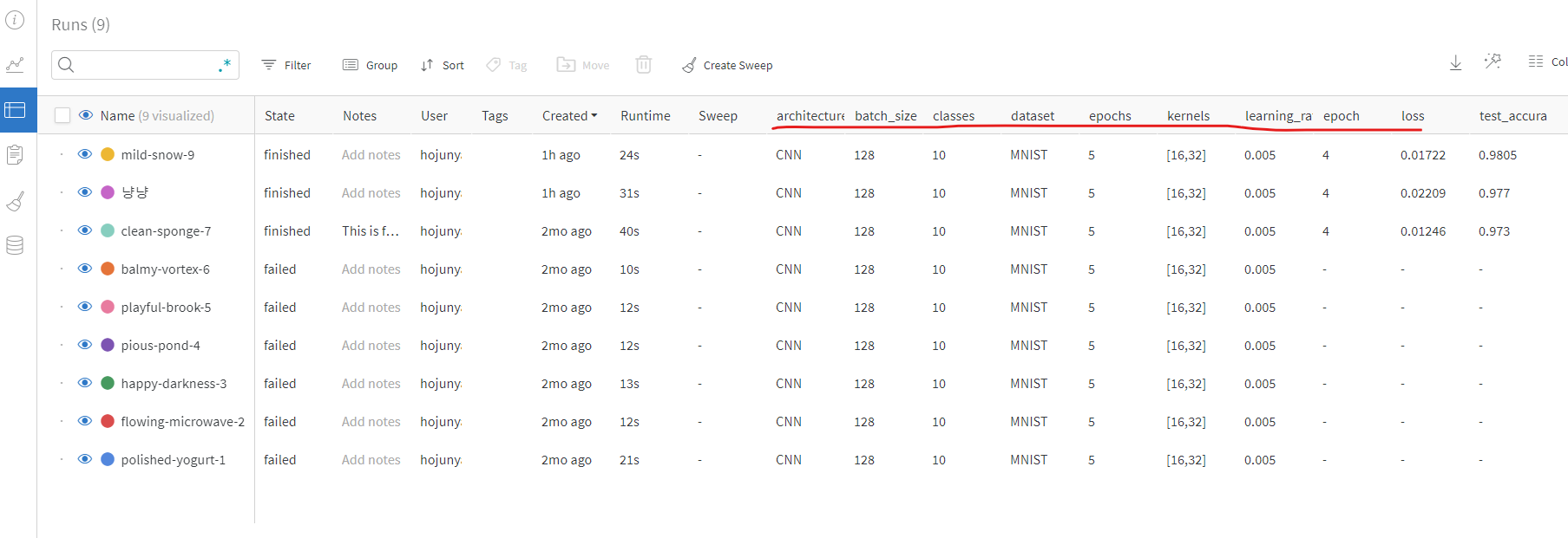
위 그림에서 볼 수 있듯 table로 항목들 살펴보면 column들에 config 항목들이 추가되어 있는것을 확인할 수 있다. 좌측의 clean-sponge-7, playful-brook-5 등은 동일한 repository에서 진행한 여러 다른 실험 결과들이다.
def model_pipeline(hyperparameters):

    # tell wandb to get started
    with wandb.init(project="pytorch-demo", config=hyperparameters):
      # access all HPs through wandb.config, so logging matches execution!
      config = wandb.config

      # make the model, data, and optimization problem
      model, train_loader, test_loader, criterion, optimizer = make(config)
      print(model)

      # and use them to train the model
      train(model, train_loader, criterion, optimizer, config)

      # and test its final performance
      test(model, test_loader)

    return model

def make(config):
    """ Training 할 때 데이터 지정하고, setting 여러개 하는거 여기서 다 하는 느낌임
    위에서 지정한 환경설정 관련 데이터가 여기서 초기화 하는데 활용됨

    """
    # Make the data
    train, test = get_data(train=True), get_data(train=False)
    train_loader = make_loader(train, batch_size=config.batch_size)
    test_loader = make_loader(test, batch_size=config.batch_size)

    # Make the model
    # 위에서 설정한 kernels, classes 정보가 여기서 쓰임
    model = ConvNet(config.kernels, config.classes).to(device)

    # Make the loss and optimizer
    criterion = nn.CrossEntropyLoss()
    optimizer = torch.optim.Adam(
        model.parameters(), lr=config.learning_rate)

    return model, train_loader, test_loader, criterion, optimizer

def get_data(slice=5, train=True):
    full_dataset = torchvision.datasets.MNIST(root=".",
                                              train=train,
                                              transform=transforms.ToTensor(),
                                              download=True)
    # equiv to slicing with [::slice]
    # Dataset 클래스(__getitem__, __len__을 가지는)를 여러개의 클래스로 쪼갠것으로 보임
    sub_dataset = torch.utils.data.Subset(
      full_dataset, indices=range(0, len(full_dataset), slice))

    return sub_dataset

def make_loader(dataset, batch_size):
    loader = torch.utils.data.DataLoader(dataset=dataset,
                                         batch_size=batch_size,
                                         shuffle=True,
                                         pin_memory=True, num_workers=2)
    return loader


# Conventional and convolutional neural network

class ConvNet(nn.Module):
    def __init__(self, kernels, classes=10):
        super(ConvNet, self).__init__()

        self.layer1 = nn.Sequential(
            nn.Conv2d(1, kernels[0], kernel_size=5, stride=1, padding=2),
            nn.ReLU(),
            nn.MaxPool2d(kernel_size=2, stride=2))
        self.layer2 = nn.Sequential(
            nn.Conv2d(16, kernels[1], kernel_size=5, stride=1, padding=2),
            nn.ReLU(),
            nn.MaxPool2d(kernel_size=2, stride=2))
        self.fc = nn.Linear(7 * 7 * kernels[-1], classes)

    def forward(self, x):
        out = self.layer1(x)
        out = self.layer2(out)
        out = out.reshape(out.size(0), -1)
        out = self.fc(out)
        return out
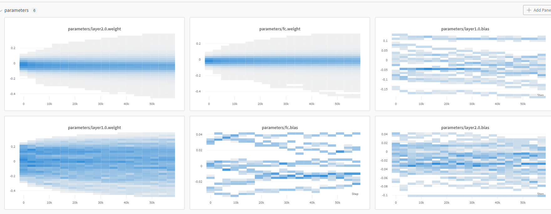
wandb.watch
wandb.watch: torch model의 gradient 등을 tracking 하기위해 사용됨- 관련 파라미터
models:(torch.Module, optional): pytorch 기반 딥러닝 모델criterion:(torch.F, optional): loss 함수log(str): gradients, parameter 중에 하나를 기입 가능하며, all을 통해 둘 다 조회 할 수도 있음
- 관련 파라미터
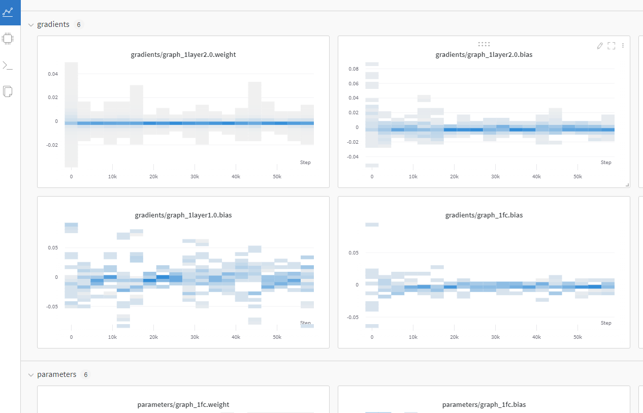
wandb 홈페이지에서 gradient, parameter 관련 그래프 조회 가능
wandb.log
wandb.log: python dictionary 타입으로 인자를 넘기며, wandb 홈페이지에서 그래프로 출력하고 싶은 값 들을 적으면 됨- 관련 파라미터
step:(int, optional): 몇 step마다 그래프로 찍을 것인지 나타냄. 값이 작을수록 촘촘한 그래프가 완성될것임
- 관련 파라미터
- wandb의
watch,log활용됨- watch: log_freq마다 gradient, parameter 로그 남기는데 활용됨
- log: 나머지 값들 로그 남기는데 활용됨
def train(model, loader, criterion, optimizer, config):
    # Tell wandb to watch what the model gets up to: gradients, weights, and more!
    wandb.watch(model, criterion, log="all", log_freq=10)

    # Run training and track with wandb
    total_batches = len(loader) * config.epochs
    example_ct = 0  # number of examples seen
    batch_ct = 0
    for epoch in tqdm(range(config.epochs)):
        for _, (images, labels) in enumerate(loader):

            loss = train_batch(images, labels, model, optimizer, criterion)     # 흔히 pytorch 프레임워크에서 쓰이는 학습 루틴
            example_ct +=  len(images)
            batch_ct += 1

            # Report metrics every 25th batch
            if ((batch_ct + 1) % 25) == 0:
                train_log(loss, example_ct, epoch)      # gradient, parameter가 아닌 다른값들을 조회하기 함수 정의 및 사용


def train_batch(images, labels, model, optimizer, criterion):
    images, labels = images.to(device), labels.to(device)

    # Forward pass ➡
    outputs = model(images)
    loss = criterion(outputs, labels)

    # Backward pass ⬅
    optimizer.zero_grad()
    loss.backward()

    # Step with optimizer
    optimizer.step()

    return loss

def train_log(loss, example_ct, epoch):
    # Where the magic happens
    wandb.log({"epoch": epoch, "loss": loss}, step=example_ct)
    print(f"Loss after " + str(example_ct).zfill(5) + f" examples: {loss:.3f}")
wandb.save
wandb.save: 모델 가중치, log, 코드등을 저장할 수 있게 해줌.
def test(model, test_loader):
    model.eval()

    # Run the model on some test examples
    with torch.no_grad():
        correct, total = 0, 0
        for images, labels in test_loader:
            images, labels = images.to(device), labels.to(device)
            outputs = model(images)
            _, predicted = torch.max(outputs.data, 1)
            total += labels.size(0)
            correct += (predicted == labels).sum().item()

        print(f"Accuracy of the model on the {total} " +
              f"test images: {100 * correct / total}%")

        wandb.log({"test_accuracy": correct / total})

    # Save the model in the exchangeable ONNX format
    torch.onnx.export(model, images, "model.onnx")
    wandb.save("model.onnx")
- 실행!
# Build, train and analyze the model with the pipeline
model = model_pipeline(config)
wandb version 0.12.16 is available!  To upgrade, please run:
$ pip install wandb --upgrade
Tracking run with wandb version 0.12.11
Run data is saved locally in <code>d:\Work\Study\wandb\wandb\run-20220517_200748-2gveead3</code>
Syncing run <strong><a href="https://wandb.ai/javis-team/pytorch-demo/runs/2gveead3" target="_blank">mild-snow-9</a></strong> to <a href="https://wandb.ai/javis-team/pytorch-demo" target="_blank">Weights & Biases</a> (<a href="https://wandb.me/run" target="_blank">docs</a>)<br/>


ConvNet(
  (layer1): Sequential(
    (0): Conv2d(1, 16, kernel_size=(5, 5), stride=(1, 1), padding=(2, 2))
    (1): ReLU()
    (2): MaxPool2d(kernel_size=2, stride=2, padding=0, dilation=1, ceil_mode=False)
  )
  (layer2): Sequential(
    (0): Conv2d(16, 32, kernel_size=(5, 5), stride=(1, 1), padding=(2, 2))
    (1): ReLU()
    (2): MaxPool2d(kernel_size=2, stride=2, padding=0, dilation=1, ceil_mode=False)
  )
  (fc): Linear(in_features=1568, out_features=10, bias=True)
)


  0%|          | 0/5 [00:00<?, ?it/s]


Loss after 03072 examples: 0.470
Loss after 06272 examples: 0.261
Loss after 09472 examples: 0.142
Loss after 12640 examples: 0.113
Loss after 15840 examples: 0.045
Loss after 19040 examples: 0.114
Loss after 22240 examples: 0.046
Loss after 25408 examples: 0.030
Loss after 28608 examples: 0.111
Loss after 31808 examples: 0.060
Loss after 35008 examples: 0.026
Loss after 38176 examples: 0.036
Loss after 41376 examples: 0.048
Loss after 44576 examples: 0.016
Loss after 47776 examples: 0.010
Loss after 50944 examples: 0.016
Loss after 54144 examples: 0.066
Loss after 57344 examples: 0.017
Accuracy of the model on the 2000 test images: 98.05%
Waiting for W&B process to finish... (success).
VBox(children=(Label(value='0.001 MB of 0.112 MB uploaded (0.000 MB deduped)\r'), FloatProgress(value=0.008004…
Run history:
| epoch | ▁▁▁▃▃▃▃▅▅▅▅▆▆▆▆███ |
| loss | █▅▃▃▂▃▂▁▃▂▁▁▂▁▁▁▂▁ |
| test_accuracy | ▁ |
Run summary:
| epoch | 4 |
| loss | 0.01722 |
| test_accuracy | 0.9805 |
Synced mild-snow-9: https://wandb.ai/javis-team/pytorch-demo/runs/2gveead3
Synced 6 W&B file(s), 0 media file(s), 0 artifact file(s) and 1 other file(s)
Find logs at: .\wandb\run-20220517_200748-2gveead3\logs
- 위 출력을 통해 나오는 링크를 들어가면 wandb와 연결되며 web을 통해 gradientes, parameters, 지정한 값 들에 대한 변화도 등을 볼 수 있다
Sweap을 통한 하이퍼 파라미터 튜닝
PREVIOUS경제